BycatchEstimator User Guide
Elizabeth A. Babcock
2025-12-29
UserGuide2.RmdIntroduction
The BycatchEstimator tool estimates total bycatch,
calculated by expanding a sample, such as an observer data set, to total
effort from logbooks or landings records. The bycatch estimates are made
with either a generic model-based bycatch estimation procedure, or
common design-based bycatch estimation methods (e.g. stratified ratio
estimator).
All bycatch estimation methods essentially estimate total bycatch as the sum over all the strata (i, e.g. years, areas, seasons), of the bycatch rate r estimated from a sample of the fishery (e.g. observer data), times the total effort E estimated from fish landings records or logbook data:
Design-based methods calculate the bycatch rate directly from the observer data with a formula (See below), while model-based estimators use a generalized linear model (GLM) to estimate a predicted bycatch rate to use in the expansion. Models can allow for more variables to be included, such as, for example, information about the habitat of the bycatch species, which may improve precision of bycatch estimates. However, model-based and design-based estimators often produce similar estimates, so that the simpler design-based estimates are sufficient in many cases.
The workflow for using BycatchEstimator is:
- Install the code and test that everything works properly by running an example.
- Run the
bycatchSetupfunction to produce data summaries and plots, to make sure that your data are appropriate for bycatch estimation. - Run either
bycatchDesignfor design-based estimators, orbycatchFitfor model-based estimators, or both. - Use the output figures and tables directly, or if desired, use the
loadOutputsfunction to input the model runs back into R for more advanced analysis. - Validate results if possible.
This user guide provides both detailed information on how to use the tool, and some general guidance on bycatch estimation.
Installing the code
The code runs best in RStudio. Before running the code for the first time, install the latest versions of R (R Core Team (2020)) and RStudio (RStudio Team (2020)). The following libraries are used: tidyverse, ggplot2, MASS, lme4, cplm, tweedie, DHARMa, tidyselect, MuMIn, gridExtra, pdftools (if pdf output is selected), foreach, doParallel, reshape2, glmmTMB, GGally and quantreg (Wickham et al. (2019); Wickham (2016); Venables and Ripley (2002); Bates et al. (2015); Zhang (2013); Dunn and Smyth (2005); Hartig (2020); Henry and Wickham (2020); Barton (2020); Auguie (2017); Wickham and Pedersen (2019); Iannone, Cheng, and Schloerke (2020); Ooms (2020);Microsoft and Weston (2020);Corporation and Weston (2020); Wickham (2007); Brooks et al. (2017);Schloerke et al. (2024); Koenker (2021)). The output figures and tables are printed to the user’s choice of an html or pdf file using RMarkdown and the knitr library(Xie (2025)). To use pdf outputs, you must have a LaTex program installed, such as TinyTex (Xie (2019), Xie (2021), Xie (2025)). For a quick start guide with example data, see the GitHub page (https://github.com/ebabcock/BycatchEstimator). For more help with installation issues, see the Installation Guide https://ebabcock.github.io/BycatchEstimator/articles/InstallationGuide.html. The following code will load the libary from GitHub using devtools (Wickham et al. (2022)).
# install.packages("devtools")
#devtools::install_github("ebabcock/BycatchEstimator")
library(BycatchEstimator)
library(MuMIn)
Data specification
The function bycatchSetup sets up the data for analysis
and provides data checks, summaries and warnings. This function takes as
input a sample from the fishery, hereafter referred to as observer data
although it could come from some other source, and a data set of total
effort, hereafter referred to as logbook data, although it could be from
any source as long as there are records of all fishing effort in the
fishery. This function must be run before running either
bycatchDesign or bycatchFit.
setupObj<-bycatchSetup(
  obsdat = obsdatExample,
  logdat = logdatExample,
  yearVar = "Year",
  obsEffort = "sampled.sets",
  logEffort = "sets",
  obsCatch = "Catch",
  catchUnit = "number",
  catchType = "catch",
  logNum = NA,
  sampleUnit = "trips",
  factorVariables = c("Year","EW","season"),
  numericVariables = NA,
  EstimateBycatch = TRUE,
  baseDir = getwd(),
  runName = "Simulated",
  runDescription = "Simulated example species",
  common = "Simulated species",
  sp = "Genus species",
  reportType = "html"
)
The observer data should be aggregated to the appropriate sample unit, such as trips or sets, so that each row corresponds to one sample unit. Effort must be in the same units in both data sets (e.g. sets or hook-hours). The logbook data may be aggregated to sample units, or it may be aggregated further, as long as it includes data on all stratification or predictor variables. For example, the logbook data can be aggregated by year, region and season if those are the stratification variables, or each row can be one sample unit. If the logbook data are aggregated, there must be a column, with a name specified in logNum, giving the number of sample units per row in the logbook data (logNum=NA means all rows on the logbook data are one sample unit). This information on the number of sample units is needed for the variance calculations. If any environmental variables, such as depth, are included, the observed and logbook data probably both have to be entered at the set level.
The observer data should have columns for year and the other predictor (for models) or stratification (for design-based) variables, the observed effort and the observed bycatch or catch per trip of each species to be estimated. The logbook data must also have columns for Year and the other predictor variables, and the total effort in the same units (e.g. sets or hook-hours) as the observer data. If there are any NA values in any of the variables, those rows will be deleted from the observer data set. Any NA values in the logbook dataset will cause the function to stop with an error message. There should be no NA values in the logbook data, because this dataset should be a complete accounting of all effort.
Any variables you intend to use in analysis should be entered in the
character vectors named factorVariables or numericVariables. Note that
design-based methods only work for categorical variables. Year is
interpreted as a factor in the design-based methods whether it is
numerical or factor. For model-based methods, Year may be either a
number or a factor. Note that there is an input “yearVar” for the name
of the year variable in your datasets. However, this variable will be
renamed as Year (with a capital Y) in the code. If Year is not a
predictor variable in your analysis, you must still input a value for
yearVar in dataSetup, but you don’t have to use it the
analysis functions. Year should be be spelled “Year” in
numericVariables, factorVariables, and all other model inputs.
The code can be used to analyze multiple species, or disposition types (e.g. retained catch, dead discards, live releases) at the same time. This is specified by inputting a vector rather than a single value for the scientific name, common name, units of estimates, and the name of the column containing the catch data (obsCatch).All these inputs can be a single value if analyzing only one species and catch type.
This function outputs the user’s choice of an html or a pdf file, or both, named with a shortened version of the species name, catch type and “data checks”, in directories named “output” followed by the specified run name. A csv file for each species is placed in a directory named for the species, sub-directory “Setup Files”. If there are multiple species or catch types, each will have their own summary file.
There will be warning messages if there are any NA values in the data or any 0 values in the observer effort data, or if levels of a factor variable in the logbook data are not present in the observer data. The html or pdf data check file will include the warnings, a table of combinations of factors present in logdat but not obsdat (if any) and the following tables and plots.
The tables are:
Observer coverage levels in both sample units (rows in the observer data) and effort (sum of the Effort columns).
A summary table by Year with number of observed and total effort units, number of positive observations of the species, number of outliers (defined as CPUE data points more than 8 standard deviations from the mean), and a simple unstratified ratio estimator estimate of the catch (See Appendix for details).
Figures comparing logbook and observer effort are:
Barplots and histograms of sum of total effort in the whole fishery and the observed sample across the levels of each categorical and numerical variable.
Pairs plots showing the overlap of observer and total (logbook) effort across pairs of categorical or numeric variables. (Categorical variables with more than 15 levels are converted to numerical to plot).
Figures showing catch in the observer data are:
Barplots of presence and absence of the bycatch species by year and by level of categorical and numeric variables.
Barplots of total catch the bycatch species by year and by level of categorical and numeric variables.
Violin plots and scatterplots of catch per sample unit, across categorical and numeric variables.
Violin plots and scatterplots of catch per unit effort (CPUE), across categorical and numerical variables.
Note that records with NA in any of the variables in the observer data, including the catch or effort variable, are excluded from the analysis and not included in the estimated sample size in the tables and figures. If there are many NAs and your sample size is low, you may want to exclude the variable from analysis or impute the missing values.
When looking at the tables and plots, check that the observer data spans roughly the same values of variables as the observer data. Design-based estimators will assume that catch is zero in strata (i.e. combinations of predictor variables) with no observer data, unless you set up the pooling options described below.
Model-based estimation methods work best of there are non-zero catches across all levels of each factor variable. Numeric variables can introduce bias if the observed data does not include the full range of values in the whole fishery. Also, look for non-linear trends in the relationship between CPUE and the numerical variable. A numeric variable will be treated as a simple linear regression in the models. If the relationship looks non-linear, you may want to consider a polynomial regression (see below). Also, check for instances of very high CPUE. This may happen if a catch occurs in a set/trip with low recorded effort, and these outliers may bias the results. In general, model-based methods are very sensitive to outliers, which are often errors in the data that should be cleaned up. If there are any zeroes values of Effort in the observer data (which is not possible), these should be corrected before doing model-based analysis.
NA values in the logbook data cause the code to stop with an error message. Values of effort and all predictor variables are needed for the entire fishery so that the total bycatch will be estimated correctly. If your total effort (logbook) data are missing values of some variables for a component of the fishery (e.g. a gear type or some years), consider excluding that part of the fishery from the bycatch calculations, and reporting bycatch only for the part of the fishery with complete effort data. If missing values are scattered throughout the dataset, consider filling in the missing values with reasonable numbers. For example, if some sets are missing data on the effort in number of hook-hours, you could replace the NAs with the mean effort (e.g. mean number of hook-hours per set if that is the unit of effort). Imputing the missing values is preferable to excluding effort from the fishery, because deleting the missing records implies that those sample units have no bycatch. Similarly, if the value of a categorical variable like gear type is missing, the NAs could be filled with the most common gear type, or with a random choice of gear type. These imputation methods will not cause bias if they number of imputed values is fairly small.
Design-based estimators
This section provides guidance on the function
bycatchDesign and using design-based estimators.
bycatchDesign(
setupObj = setupObj,
designScenario = "withPooling",
designMethods = c("Ratio", "Delta"),
groupVar = "Year",
designVars = c("Year","season","EW"),
designPooling = TRUE,
poolTypes=c("adjacent","all","none"),
pooledVar=c(NA,NA,NA),
adjacentNum=c(1,NA,NA),
minStrataUnit = 1
)
The function takes the output of bycatchSetup
(e.g. setupObj) as an input, which must have been run on the same day,
along with specifications for the design-based estimators. You may run
multiple scenarios (e.g. different pooling specifications) from the same
setupObj, by specifying a scenario name (designScenario), which will be
included in the output file names. The design-based methods available
are a stratified ratio estimator Rao
(2000) or the design based delta-lognormal estimator of Pennington (1983). To use design-based
estimators, specify them as a character vector. For example,
designMethods =c(“Ratio”,“Delta”) will calculate both estimates. The
total bycatch estimates are made at the stratification variables defined
by the user in the vector called designVars, which must be categorical
variables. Annual summaries are produced by summing across strata within
years. If you want to produce the output plots across some variable
other than Year (e.g. 2-year periods), specify the name of this variable
with groupVar.
To deal with strata that have no observations or few observations, the user may request pooling (designPooling=TRUE), and specify the minimum number of sample units needed to avoid pooling. If pooling, the total bycatch is estimated for the observer and logbook data specified by the pooling scheme for each stratum (i.e. combination of variables) and then allocated to the stratum according to the fraction of the logbook effort in the pooled data that is in the stratum of interest. Unpooled estimates are used for strata with sufficient data. Variances are also allocated to the stratum of interest based on the fraction of total effort. See Brown (2001) for details of one potential pooling scheme. If pooling is requested, the strata will be pooled in the order of designVars. Three additional vectors are needed to define how the pooling works: poolTypes, which says whether the variable should be pooled across “adjacent” levels (for Year only), “all” values, a new variable “pooledVar” (e.g. season rather than month) or “none” if the levels of a variable should always be kept separate; pooledVar which specifies the new variable for pooling for the pooledVar pooling method; and adjacentNum which specifies the number of adjacent years to include for the adjacent year method (e.g. 1 to include both the previous and following year). Each of these vectors must be the same length as designVars. You must also specify the minimum number of sample units in a stratum to require pooling.
This function produces the user’s choice of a pdf or html file with bycatch estimates for each species and catch type, labelled with the designScenario and species name plus “design results”. The file includes a table with the total estimates by year for each method, along with standard errors, a figure showing the estimates by year with 95% confidence intervals. If pooling was requested, there is a barplot showing the number of strata pooled in each Year to each variable in designVars, also indicating the number of strata that have not acheived the specified minimum number of sample units.
The outputs are also given in .csv files in a folder labeled “Design outputs”. The estimates are in columns called ratioMean, ratioSE, deltaMean and deltaSE in the file labelled DesignSummary (by year) and the file labelled DesignStrata (by stata). If pooling was requested, a csv labelled “pooling” gives the number of sample units in the strata with and without pooling, etc. See details on outputs in the Appendix.
In general, if there are any combinations of the stratification variables (designVars) which do not exist in the observer data but do exist in the logbook data, you should consider at least some pooling. Without pooling, the model will assume there is no bycatch in the unsampled strata, so that, if there are many stratification variables, the total bycatch could be under-estimated substantially. You can experiment with different pooling schemes and see if they give very different results, by giving them different designScenario names.
Note that leaving out a variable from the list of designVars is equivalent to always pooling over all levels of that variable. If the observer program allocates observer sampling effort by a stratified random design, in which the observer coverage level varies by strata, it is usually necessary to include all the stratification variables in the design. For example, if observers are allocated so that roughly equal numbers of sets are covered in each stratum defined by gear, year, area and season, then strata with more fishing effort will have lower observer coverage rates. In this case, all the stratification variables should be included in the design-based estimators, so that pooling can be used only where needed. On the other hand, if observers are allocated randomly across the whole fishery (a simple random design) then there is no need to include any stratification variables, as the average bycatch rate across the sampled part fo the fishery will be representative.
If including multiple stratification variables is necessary, but the sample sizes are small enough to require pooling, the pooling strategy should be developed to pool only across strata that have similar bycatch rates. The CPUE plots by level of each variable in the Data Checks are useful for this. For example, if seasons are very different, but years are similar within seasons, then it makes sense to use adjacent year pooling. Similarly, areas that are similar to each other can be pooled. For example, if there are 10 fishing areas, you could group them into 2 fishing zones (e.g. zone 1 is areas 1-5, zone 2 is areas 6-10), and use the pooledVar feature to pool within zones if needed. Something like the following would pool on adjacent years and areas within zones:
designVars = c("Year","area")
designPooling = TRUE
poolTypes=c("adjacent","pooledVar")
pooledVar=c(NA,zone)
adjacentNum=c(1,NA)
The minimum number of sample units needed to avoid pooling can also be adjusted. In general, the pooling should require enough sample units that the estimated bycatch rates are generally above zero in the pool. For example, if the species is caught in one set out of 10, then a minimum sample unit of 10 might work. On the other hand, more pooling will have the effect of smoothing out the differences between strata, which may not be desirable if the purpose of the study is to compare strata. Experiment with different levels of pooling and see if the pooling makes a difference in the estimates, using a different designScenario name for each version. Of course, increasing the observer coverage level so that pooling is not needed would provide the best bycatch estimates.
Model specification
Model-based analysis to estimate total bycatch and/or to generate an
abundance index is done with the function bycatchFit
bycatchFit(
  setupObj = setupObj,
  modelScenario = "s1",
  complexModel = formula(y~Year+season),
  simpleModel = formula(y~Year),
  indexModel = formula(y~Year),
  modelTry = c("Tweedie","Lognormal","Delta-Lognormal","Delta-Gamma", "TMBnbinom1","TMBlognormal",
                          "TMBnbinom2","TMBtweedie","Normal","Binomial","NegBin", "TMBgamma","Gamma",
                          "TMBbinomial","TMBnormal","TMBdelta-Lognormal","TMBdelta-Gamma","Poisson","TMBpoisson")[c(7,8,16)],
  randomEffects = NULL,
  randomEffects2 = NULL,
  selectCriteria = "BIC",
  DoCrossValidation = TRUE,
  CIval = 0.05,
  VarCalc = "Simulate",
  useParallel = TRUE,
  nSims = 100,
  plotValidation = FALSE,
  trueVals = NULL,
  trueCols = NULL,
  reportType = "html"
)
## [1] "1 Simulated species, catch, complete, 2025-12-29 19:48:45.63186"The user specifies which potential predictor variables to use and what potential error distribution models (e.g. negative binomial, delta-lognormal) to use. The function uses information criteria to pick the best set of predictor variables for each error distribution model automatically using the information criterion. For the best model in each group, total bycatch estimates and model diagnostics are generated. To provide guidance on choosing between observation error model groups, cross-validation is available. This section explains how to run the model and interpret the results. The following section gives more technical details and guidance on model selection.
To use this function, specify the input data object generated by
bycatchSetup. You may run more than one scenario from the
same setupObj, by specifying “modelScenario”. The character vector
“modelTry” indicates both the potential observation error distributions
to try and which functions to use in the fitting. Options are: “Tweedie”
from the cplm
library,“Lognormal”,“Delta-Lognormal”,“Delta-Gamma”,“Normal”,“Binomial”,“Poisson”
and “Gamma” from the ordinary glm and lm
functions, “NegBin” from the MASS library’s glm.nb
function, and “TMBnbinom1”,“TMBlognormal”, “TMBnbinom2”,“TMBtweedie”,
“TMBgamma”, “TMBbinomial”, “TMBnormal”, “TMBpoisson”,
“TMBdelta-Lognormal” and “TMBdelta-Gamma” from glmmTMB). A binomial
model will be tried if it was requested, or if either a delta-lognormal
or delta-Gamma model were requested, since delta models have a binomial
component. Note that the model outputs with the same funtional form
(e.g. Tweedie) should be the same whether using glmmTMB or other
functions. The negative binomial 2 in TMB is the same as the negative
binomial in glm.nb. To get faster results, use glmmTMB for all model
fitting.
Give the formulas for the most complex and simplest set of predictor
variables to be considered within each model group. These should be in
the format of R formulas (e.g. formula(y~Year)), with y on the
left-hand side of the formula. The year variable must be called Year
(capital Y), whatever it is called in the actual data (entered in
yearVar). If the simplest model requires stratification variables other
than Year, summaries of the predicted bycatch at the level of these
stratification variables will be printed to .csv files, but will not be
plotted. The user-specified simplest model will often include Year, and
can also include, for example, stratification variables that are used in
the observer program sampling design. If Year is not in the simplest
model (e.g. simplest model is the null model y~1), the model still
produces bycatch estimates in each year, which can vary from one year to
the next if effort changes. If an abundance index is requested, it will
be calculated including all the variables requested in indexVars, to
allow for different indices for different stratification variables if
desired (e.g. different spatial areas). All the variables used in the
model must have been included in either numericVariables or
factorVariables in bycatchSetup, and they retain this
classification.
The variables in the simplest and most complex model are interpreted as fixed effects. Any desired random effects can be entered as a character vector (e.g. randomEffects=“Year:area”). In the case that any delta models are used, there can be separate random effects for the binomial model (randomEffects) and abundance when present model (randomEffects2). If there are any random effects, all fitting will be done in glmmTMB. Random effects, if any, will be included in all models during model selection. This may be useful for including a trip effect in a set-by-set analysis, for example, or for including a Year:area interaction as a random effect when calculating indices.
Specify which information criterion to use in narrowing down the predictor variables to use in each observation error model group; or use the default of BIC. Model selection is done with dredge function in the MuMIn library(Barton (2020)) based on the user’s choice of information criteria (AICc, AIC or BIC) and considering all models between the simplest and most complex. The model with the lowest value of the information criterion is chosen as best within each observation error group.
Specify whether to do cross validation to choose between observation error models. The best candidate models in each observation error group are then compared using 10-fold cross validation, to see which observation error model best predicts CPUE. Note that information criteria cannot be used directly to compare, for example, delta-lognormal to negative binomial or Tweedie, because the observation error models have different y data. However, the models can be used to predict CPUE directly, and these predictions can be compared with cross validation. The best model according to cross validation is the one with the lowest root mean square error (RMSE) in the predicted CPUE and the mean error (ME) closest to zero, excluding from consideration models that do not fit well according to criteria described below. Note that this model selection using information criteria and cross validation is only intended as a guide. The user should also look at the information criteria across multiple models, as well as residuals and other diagnostics, and may want to choose a different model for bycatch estimation or abundance index calculation based on other criteria, such as the design of the observer sampling program. Also, the code only does one draw of the 10-fold cross-validation, so that, for small sample sizes, different model runs may give different cross-validation results.
For the best model in each observation error model group, the total
bycatch is estimated by predicting the catch in all logbook trips (i.e.,
the whole fishery) from the fitted model and summing across trips. If
includeObsCatch is FALSE (the default), the bycatch will be predicted
across all the logbook data, There is an option, using
includeObsCatch=TRUE, to only predict bycatch from unobserved effort
(i.e. trips or sets not sampled by observers, and for sampled trips or
sets, only the effort not sampled by the observer) and calculate total
bycatch as the observed bycatch plus the predicted bycatch in unobserved
effort. This only works if it is possible to match the observed trips or
sets to the logbook trips or sets, and the amount of observed effort in
a sample unit is always less than or equal to the amount of total
effort. For fisheries with high observer coverage (e.g. 20% or more),
predicting bycatch from only unobserved effort would be preferred,
because treating the whole fishery as unobserved might overestimate the
variance. To use this option, there must be a column with the same name
in both obsdat and logdat (matchColumn), such as trip number or set
number, that can match all observations in obsdat to logdat. If the
observer sampled only part of the effort (e.g. they sampled only some
sets in a trip), then bycatch will be predicted for the logdat effort
minus the obsdat effort for observed sample unit. If includeObsCatch is
TRUE, bycatchFit will give warnings if, for example, sample
units in the observer data are not found in the logbook data, or the
observed effort is more than the logbook total effort in any sample
units. This option works in the simulated example data, but can be
difficult to set up with real data, and requires a lot of data cleaning,
to make the observer and logbook data consistent.
The function may be slow (more than an hour) if you have a large data set. If the variable useParallel is TRUE and your computer has multiple cores, the dredge function will be run in parallel. This greatly speeds up the calculations. If you have trouble getting this to work, set useParallel to FALSE.
Finally, if you have information on total bycatch in each year to
validate your estimates, for example in a simulation study, fill out the
arguments plotValidation, trueVals,
trueCols. Otherwise, leave these arguments out, or set
themto FALSE, NULL and NULL, respectively. To include validation data,
trueVals should be set equal to a character string
containing a filename (with complete path) for a file containing a
column labelled “Year”, and columns with the total bycatch in each year,
with names specified in trueCols. For multiple species,
trueCols can be a vector giving the names of all the column
for each species in order.
After the function runs, the summary model results file (html or pdf), named with the species name and model scenario (e.g. BlmarlnCATs1Modelresults.html) is printed in a folder labelled with the species common name. The file begins with text describing the model inputs and some basic information about which models were fit successfully. The diagnostics and model details are explained more fully below.
For all models together, the file includes:
The model comparison table, showing the best model according to the information criteria, along with a column on the cause of model failure, if any. If cross-validation was requested the mean values of the ME and RMSE are included.
The results of tests of whether the residuals are consistent with each model.
Parameters from the fitted models, including the scale (variance or the estimated scaling parameter depending on the model type) along with the total log likelihood and residual degrees of freedom.
A figure of bycatch across years, with confidence intervals.
A figure of the abundance indices across years, if requested, with confidence intervals.
Boxplots of the cross validation metrics across folds, if cross-validation was requestd.
For each model type, the file includes:
The model selection table from the MuMIn dredge function.
Ordinary and quantile residual figures.
Observed vs. predicted values figures.
The figures showing the total catch with confidence interval.
If requested, an abundance index.
These results may be all that is needed. However, if you want to look more closely at a specific model result, whether or not it was selected by the information criteria and cross validation, all the outputs are printed to .csv files in the folders listed for each species, in a folder called “Fit files”. These files are:
Model Selection. The MuMIn dredge model selection table.
Annual Summary. The estimated total bycatch, standard errors and confidence intervals for the model.
Stratum Summary. The estimated total bycatch, standard errors and confidence intervals for the model at the variables in simpleModel.
Annual Index. The annual abundance index if requested.
Details and guidance on using models
The bycatchFit function provides many options for the
observation error model groups (modelTry) to allow users flexibility in
setting up models. However, many of these models (e.g. normal, Poisson)
are unlikely to be effective. In practice, negative binomial (1 or 2),
delta-lognormal or Tweedie work for most applications, and the glmmTMB
versions run quickly. This section provides more details on how the
model fit and selection works, with guidance for selecting models.
GLM model types
Generalized linear models (GLM) vary on whether they assume the y data will be 0 and 1 (binomial), counts (negative binomial), or real numbers (all others), how they model the mean and how they model the variance of the data. When the user selects a model, the code automatically sets up these details (e.g. link functions, response variables, offsets) as explained here.
| Distribution | Response(y) | Link | Mean | Variance |
|---|---|---|---|---|
| CPUE,real | identity | |||
| CPUE,real, | log transformed | |||
| CPUE,real, | ||||
| CPUE,real, | ||||
| presence/absence (0,1) | ||||
| Catch,integer, | ||||
| Catch,integer, | ||||
| Catch,integer, |
The code takes Catch and Effort as inputs and calculates CPUE as Catch/Effort in each sample unit. Presence is zero if Catch is zero and 1 otherwise.
The binomial models presence/absence data, so it is only used to estimate the probability of presence, not the expected CPUE. For binomial, the mean probability of a positive observation is modeled with a logit link, meaning that the log of the odds of a positive observation is predicted by the linear model. This model may be used on its own to estimate bycatch of very rare species where only one is ever caught at a time, and it is also used to model positive versus zero observations in the delta models (see below).
The negative binomial using the glm.nb function from the MASS library (Venables and Ripley (2002)) or nbinom2 from the glmmTMB library(Brooks et al. (2017)) are the ordinary negative binomial, in which the variance is: where is an estimated parameter. For nbinom1, the variance is defined as: where is an estimated parameter. This version of the negative binomial model, which is equivalent to a quasi-Poisson model, gives somewhat different results from the other negative binomial models. The estimated values of or are given in the “scale” column in the parameter summary table.
The negative binomial models predict integer counts, so they are appropriate for modeling bycatch in numbers per sample unit. To model catch per unit effort (CPUE) when each sample unit(e.g. set) might have a different amount of effort (e.g. hook-hours) it is necessary to include effort as an offset in the model. We use a log link for all negative binomial models, so that the model predicts:
where is the catch in sample unit in the observer data, is an example linear predictor with an intercept and a slope, and the offset is the log of the effort in each trip. This is algebraically equivalent to modeling CPUE as a function of the same linear predictors, e.g. The model can then be used to predict CPUE by inputting Effort=1, and to predict catch by inputting the Effort in a sample unit. The code sets up the offset automatically, so you don’t have to put it in simpleModel or complexModel. However, the best models shown in the output tables will show the full formula in R formula format, e.g. the formula above would be , where 1 indicates the intercept, and the offset is distinguished from predictor variables by the keyword “offset”. Negative binomial models work well, even for very rare species, if the data are counts of the numbers of animals caught, because the model can handle large numbers of zero observation with a low estimated mean. To allow negative binomial models to also be used with catch or bycatch measured in weight (i.e. non-integer values), the code rounds the catches to integers before running this model. If any of the catches are less than 0.5, they will be rounded to 0, so you might want to change the scale if using negative binomial models (e.g., multiply by 10).
The Poisson distribution, available from modelTry = “Poisson” or “TMBpoisson” works the same as the negative binomial except that it does not have an estimated scale parameter, and it defines the variance as equal to the mean. The Poisson is appropriate for completely random count data that are not either clumped or overdispersed. It generally does not work as well as the Negative Binomial, but it is included for comparison. It may be worth using if the scale parameter in negative binomal 1 or 2 implies that the variance is similar to the mean (i.e. a large value of the scale parameter in nbinom2, or a small value near zero in nbinom1 implies the variance is close to the mean).
The Tweedie distribution (“Tweedie” or “TMBtweedie” in modelTry) is a generalized function that estimates a distribution similar to a Gamma distribution, except that it allows extra probability mass at zero. It is thus appropriate for either continuous or integer data with extra zeros. It uses a log link, and, in addition to the linear predictor for the log(mean) of the CPUE, it estimates an index parameter and dispersion parameter which together determine the shape of the distribution. The variance is .
Delta-lognormal models work by applying a binomial model to the presence or absence (0,1) of the bycatch species in the each sample unit to estimate the probability of presence. Then, the mean CPUE conditional on the species being present is calculutated by fitting a lognormal or Gamma model to the positive observations only. For the delta lognormal models, the CPUE is log transformed, and the mean CPUE for positive observations is modeled for positive data only. For the delta-Gamma method, the log link is used to model the positive CPUE values. Because the the lognormal or Gamma component is fitted to the positive CPUE observations, it is possible to have some levels of the factors that do not have any data (i.e the species was never observed in some strata). In this case, you will see a warning and some variables may be dropped from the model. If some years don’t have data and year is a predictor variable, the delta models will not be applied. Delta models do not work for very rare species and small sample sizes because they require at least some positive observations across the range of variables for the lognormal or Gamma models to be meaningful.
Simple normal, lognormal and Gamma options are also available. Lognormal and Gamma models are run on all the CPUE data, including zeros, after adding a constant of 0.1, which is subtracted when making predictions. These models are unlikely to work will with rare species, but are included for comparison.
Model selection with information criteria
Within each observation error model group, the information criteria
are used to find the best model. The MuMin dredge function
does this by fitting all nested models between the most complex and the
simplest. For example, if complexModel was
,
which is the model with Year, season and their interaction
,
and simpleModel was the Null model
,
then the models included would be:
The recommended model selection criterion is BIC because BIC is less likely to prefer overly complex models when the sample size is large (Burnham and Anderson (2004)). Information criteria work by weighing the tradeoff between model fit and model complexity. The AIC is where L is likelihood, is model deviance, and is the number of parameters. A lower deviance (higher likelihood) implies better model fit. However, the complexity penalty means that an added parameter (e.g. another predictor variable coefficient) must reduce deviance by more than 2 units to improve the fit enough to be worth the extra parameters. BIC is where is total sample size. Thus, the complexity penalty increases with sample size. This is desirable for large datasets where, with AIC, the most complex proposed model would almost always be preferred even if it explained very little of the model deviance.
The MuMin summary table (in both the model summary file and a
separate CSV) includes all the information criteria for each model that
was considered, as well as model weights calculated for the information
criterion the user specified,
,
where delta
is the difference in information criteria between model
and the best model. Model weights sum to one and indicate the degree of
support for the model in the data (Barton
(2020)). The best model will have the highest weight and the
lowest
.
But, in some cases other models may also have strong support, and should
perhaps be considered, particularly if they are simpler. The current
version of the code does not use MuMIn’s model averaging function, but
this may be worth considering if several models have similar weights.
The model selection table also includes the other information criteria,
so you can see if they are consistent. We also provide a value of pseudo
in the model output table. This is calculated using the
r.squaredGLMM function (Barton
(2020)), and can be interpreted as a rough measure of the
variance explained by the model. However, note that high
values may not be needed for bycatch estimation;
measures how accurately each sample unit’s bycatch can be predicted, but
the total bycatch is summed over many sample units, and may be quite
accurate even if the variation between sample units is not well
explained.
When deciding which sets of predictor variables to use, keep in mind the following. If the observer program is set up with a stratified random sampling design, meaning that the observer coverage level varies between stratify defined by the factor variables of Year, area, season, geartype, etc., then all of these variables should be included in the model to avoid bias caused by oversampling strata with atypical bycatch rates. As an extreme example, suppose the observer program had allocated extra observers to a strata (a particular gear and area) in recent years because that strata was known to have higher bycatch of the species of interest. In this case, it would be necessary to include gear, season, year, area and at least some of their interactions in the model to allow the model to localize the high bycatch rates in that strata. For example, an appropriate complexModel might be . This is equivalent to
This model with all possible interactions allows each strata to have its own estimated bycatch rate, and is most similar to a design-based estimator with the same stratification variables and no pooling. Of course, it would be necessary to have data on all combinations of the variables to fit this model, which often does not happen, even with large sample sizes because not all gear types are used in all areas. An alternative approach would be to include a variable called for example gearArea that combined those two variables, which would avoid the need to estimate non-exsistent combinations. Another options is to include interactions as random effects to make them estimable (Ortiz and Arocha (2004)).
If sample sizes are small or the species is rare, it may not be possible to estimate bycatch rates in each Year separately (i.e. to include year as a factor variable in simpleModel), although annual estimates of total bycatch are often needed. One possible solution is to not require Year to be in the model, by not including it in simpleModel. For example, setting simpleModel to the null model allows the information criteria to be used to find the best model, even if it does not include Year or any other variable. The model will still produce separate estimates in each Year, because the model predicts bycatch in the recorded logbook effort, so that more effort will lead to more estimated bycatch even if the model estimates the same CPUE in all sample units. Another possible approach is to include 2-year or 3-year periods as a factor variable, rather than Year. Again, each Year will still have its own bycatch estimate, but the model predictions of bycatch rate can be estimated by a model that does not include Year specficially as a variable. Finally, Year can be input as a numeric variable. This approach can be useful to model a consistent increase or decrese over time. With a numeric Year, a model such as will estimate a linear trend across years. Polynomial regression may be a useful way to estimate more complex trends across years in data sets where not all years have enough data to estimate Year as a categorical fixed effect. This can be specified as, for example .
When considering including additional variables in the model, other than Year and any stratification variables used in the sampling design, the key consideration is whether the variable is available, and has the same interpretation, in both the observer and the logbook data. For example, an analyst might want to include a gear description variable because it influences catch rates in the observer data. However, the logbook data may not have the exact same information for all effort. In this case, even if the variable would improve the predictive skill (i.e R squared) of the model fitted to the observer data, and would be useful in CPUE standardization from the observer data, it could not be use for total bycatch estimation.
Model residuals and residual diagnostics
For the best model (according to the information criterion) in each observation error model group, both ordinary residuals and DHARMa scaled residuals are plotted (also called quantile or PIT probability integral transform residuals), and the DHARMa diagnostics are calculated (Hartig (2020)). The DHARMa library uses simulation to generate quantile residuals based on the specified observation error model so that the results are more clearly interprettable than ordinary residuals for non-normal models. DHARMA draws random predicted values from the fitted model to generate an empirical predictive density for each data point and then calculates the fraction of the empirical density that is greater than the true data point. Values of 0.5 are expected, and values near 0 or 1 indicate a mismatch between the data and the model. Particularly for the binomial and negative binomial models, in which the ordinary residuals are not normally distributed, the DHARMa residuals are a better representation of whether the data are consistent with the assumed distribution.(See the DHARMa vignette (Hartig (2020)) for a good explanation of how to interpet quantile residuals.) Both the regular residuals and the DHARMa residuals are appropriate for lognormal and Gamma models, since they model continuous data which is expected to be approximately normal when transformed by the link function. The model output file shows a table with P values for a Kolmogorov-Smirnoff test of whether the DHARMa residuals are uniformly distributed as expected, a test of over-dispersion, a test of zero-inflation (which is meaningless for the delta models, but helpful to see if the negative binomial and tweedie models adequately model the zeros) and a test of whether there are more outliers than expected.
For models to be used in further analyses, the DHARMA residuals should be uniformly distributed, as indicated by the QQUniform plot and (for small datasets) the Kolmogorov-Smirnov test of uniformity. If the DHARMA residuals show substantial over-dispersion then the model is not appropriate. In general,a well-specified model will show the points along the line in the DHARMa qqnorm plots, and points scattered between 0 and 1 with no pattern in the DHARMa residual plot. For large datasets, violations of assumptions matter less in model fitting. However, it is better to select a model group with no obvious deviations form model assumptions in the DHARMa residual plots.
When the models are fit, the code keeps track of whether the model converged correctly, or if not, where it went wrong. The model fit summary table in the model results file shows a “-” for models that converged successfully, “data” for models that could not be fit due to insufficient data (no positive observations in some year prevents fitting the delta models), “fit” for models that failed to converge, and “cv” for models that produced results with unreasonably high CVs (>10). Models that fail in any of these ways are discarded and not used in cross validation or bycatch estimation. If you get one of these errors for a model you want to use, you should check the data checking figures and tables for missing combinations of predictor variables, extreme outliers, or years with too few positive observations.
Cross validation
Cross-validaton is a method to identify models that perform well at out-of-sample prediction, meaning predicting the values of y data points that were not used to fit the original observations. Only observation error models that converged and produced reasonable results with the complete data set are used in cross validation. For example, if there were not enough positive observations in all years to estimate delta-lognormal and delta-Gamma models, then they will not be included in the cross validation.
For the cross validation, the observer data are randomly divided into 10 folds. Each fold is left out one at a time and the models are fit to the other 9 folds. The same predictor variables chosen as the best model on the full dataset will be used in each fold as for the full data set to save time. The fitted model is used to predict the CPUE for the left out fold, and the root mean square error is calculated as:
where n is the number of observed trips and y is the CPUE data in the left-out tenth of the observer data, and is the CPUE predicted from the model fitted to the other 9/10th of the observer data. The model with the lowest mean RMSE across the 10 folds is selected as the best model. Mean error (ME) is also calculated as an indicator of whether the model has any systematic bias.
Note that cross-validation is only done for one random draw of the data. To use cross-validation for model selection it would be appropriate to do more than one draw. This is only intended to diagnose large problems with model predictive ability. In practice, for many data sets the cross-validation shows that many models perform similarly, and they make very similar estimates of total bycatch.
Total bycatch calculation
For each model group, the best model, as selected by the information criteria, is used to estimate the total bycatch with the exception of the binomial, for which the model estimates the total number of positive trips. For the binomial model, the best model is used to predict probability of a positive observation in each logbook trip and these are summed to get the total number of positive trips in each year (and in each stratum if further stratification was requested). The number of positive trips is calculated because, for a very rare species that is never caught more than once in a trip, the number of positive trips would be a good estimate of total bycatch and many of the other models would fail to converge. For more common species, the estimates of total catch are more appropriate, so the results of the binomial model alone are not included in the cross validation for model comparison.
To calculate total bycatch for all other models, the model predicts the catch in each sample unit of the logbook data from the models fitted to the observer data and sums them over sample units to get the total baycatch. For all the negative binomial models, the log(effort) from the logbook trips is used as an offset in the predictions, along with the values of all the predictor variables, so that the model can predict bycatch in each logbook sample unit directly. Tweedie and normal models predict CPUE, which is then multiplied by effort. Delta-lognormal and delta-Gamma models have separate components for the probability of a positive observation and the CPUE if positive, which must be multiplied together (with appropriate bias corrections) and multiplied by effort to get the total catch. Catch in each sample is summed across sample to get the total catch in each year.
The variance of the prediction in each sample is calculated as the variance of the prediction interval, which is the variance of the estimated mean prediction plus the residual variance. The variances are then summed across sample units to get variance of the total catch estimate in each year. Because the predicted catches in each logbook trip are dependent on linear model coefficients, which are the same across multiple trips, the trips are not independent; thus, the variances cannot be added without accounting for the covariance. The variance of the total catch in each year is thus calculated either using Monte Carlo simulation, or using a delta method (described below). Users may also chose not to estimate variances for large logbook datasets where these methods will not work. In the case where only the unobserved bycatch is estimated, the observed bycatch is added to the predictions as a known constant with no variance. The delta method variance is not available for the delta-lognormal, delta-Gamma or Tweedie models using cplm, although it is available for Tweedie using glmmTMB.
For delta-lognormal models, the variance of the predicted CPUE is needed to bias-correct when converting the mean predicted log(CPUE) to mean predicted CPUE. The variance of the prediction interval for each trip is calculated as the variance of the estimated mean plus the residual variance, and this value is used in the bias correction. The total predicted CPUE is the predicted probability of a positive observation from the binomial times the predicted positive CPUE, and predicted catch is the predicted CPUE times effort. The variance of the total CPUE is calculated using the method of Lo, Jacobson, and Squire (1992).
For the Monte Carlo variance estimation method, we first draw random values of the linear model coefficients from a multivariate normal distribution with the mean and variance/covariance matrix estimated from the model. The predictions for each trip are then drawn for each draw of the parameters using the appropriate probability density function (e.g. Tweedie, negative binomial) with additional parameters (e.g. residual variance, negative binomial dispersion, Tweedie and ) estimated by the model. Trips are then summed for each year (adding the observed catch if necessary) within each draw, and the mean, standard error, and quantiles (e.g. 2.5% and 97.5% for a 95% confidence interval) are then calculated across the Monte Carlo draws. An approximation of the total variance of the predicted bycatch can also be made using a delta method. The delta method approximates the variance of a function of a variable as the derivative of the function squared times the variance of the original variable. Thus, the variance of the prediction intervals in the original data scale is calculated by pre and post multiplying the derivative of the inverse link function to the variance covariance matrix of the predicted values.
were is the variance covariance matrix for the predicted trips in the stratum on the scale of the log link, and J is the matrix of derivatives. See the function MakePredictionsDeltaVar in bycatchFunctions.R for the details for each model type. This code is partly based on the method developed by https://stackoverflow.com/questions/39337862/linear-model-with-lm-how-to-get-prediction-variance-of-sum-of-predicted-value. The delta method is not available for delta-Gamma, delta-lognormal, or Tweedie via the cplm library. For those error models, the simulation method will be used even if the delta method is selected with VarCalc.
If the logbook data is aggregated across multiple trips (e.g. by strata) the effort is allocated equally to all the trips in a row of the logbook data table for the purpose of simulating catches or estimating variances using the delta method. This allocation procedure is not needed to estimate the mean total bycatch, but it is necessary to estimate the variances correctly. When using aggregated effort, it is not yet possible to include the observed catches as known.
Grouping and aggregation in data
A final consideration in data setup for models is what to use as the sample unit. In a longline fishery, for example, bycatch estimation is often done with set-by-set data. However, because observers are allocated to vessel-trips, not sets, and sets within trips are correlated, using sets as the sample unit without modeling the within vessel-trips correlation might introduce bias in both the total bycatch and variance calculations. For an example, if the 10% of sets that are sampled are all from the same vessel-trip in the same area, then they will not be representative of the fishery. Because all the sets are similar, the estimated bycatch may be biased, and the confidence intervals will be too narrow.
One solution to this problem is to put vessel or vessel-trip in the model as a random effect. This has the effect of correctly modeling the grouping of the data withing vessel-trips, and is probably the most statistically correct way to deal with the problem. Another solution is to use trips as the sample unit. In this case, the observer data will include the some of bycatch and effort across sets in a trip, elimimating the problem of correlation between sets. This has the advantage of reducing the sample size to more correctly account for the number of independent samples (vessel-trips), so that variance esimates will be correct. This method does not work if any important variables have to be included at the set level, such as, for example, if depth zone is a stratification variable and vessel-trips may fish in more than one depth-zone. If only a few trips fish in multiple depth-zones (or other variable) then the most common one can be assigned to the trip without much loss of information. See Babcock et al. (2018) for an example where this method was used for sea turtle bycatch in shrimp trawls.
Abundance index calculation
If a user requests an annual abundance index, this is also calculated from the best model in each model group. The annual abundance index is calculated by setting all variables other than year, and any variables required to be included in the index (e.g. region or fleet) to a reference level, which is the mean for numerical variables or the most common value for categorical variables. The index is calculated by predicting the mean CPUE in each year, and its standard error is calculated as the standard error of the mean prediction. For delta-lognormal and delta-Gamma models the standard error of the prediction is calculated from the means and standard errors of the binomial and positive catch models using the method of Lo, Jacobson, and Squire (1992).
If you set EstimateBycatch to FALSE, and EstimateIndex to TRUE,
bycatchFit can estimate a CPUE abundance index from any
dataset. The dataset to be used for the index should be estimated as
“obsdat” even if it is a logbook dataset, because the model is applied
to the dataset labelled “obsdat”. For advice on CPUE standardization,
see papers by Ortiz and Arocha (2004),
Maunder and Punt (2004) and Hoyle et al. (2024).
Loading outputs for futher plotting and analysis
You may use the function load loadOutputs to read in
either the model-based or design-based results, by specifying the
runName, runDate, and character vectors of values of designScenario
and/or modelScenario. This function returns a list, including:
setupObj which the original setupObj for the run
designObjList which is the results across designScenarios including bycatchInput and bycatchOutput lists.
ModelObjList which is the results across modelScenarios including modelInput and modelOutput lists.
The runName
allYearEstimates which is a long-format data-frame with all the results of the design-based and model-based estimate from all the design and model scenarios requested. If more than one species or catchtype was run, they will all be included. There are columns for Scenario (design and model), Common (common name), Species (scientific name), CatchType, Source (the method or model used in estimation), Run (the run name), as well as Year, Total, Total Var, Total.mean, TotalLCI, TotalUCI, Total.se, Total.cv, and a column called Valid, which will be 1 for valid models or methods, and 0 for models that had some problem in the model fitting. This data-frame is appropriate for ggplot.
library(tidyverse) #for data manipulation and ggplot
#Load in both design and model based estimates
allResults<-loadOutputs(baseDir = getwd(),
                      runName= "Simulated",
                      runDate =  Sys.Date(),
                      designScenarios = "withPooling",
                      modelScenarios = "s1"
)
#Plot all together
ggplot(allResults$allYearEstimates,aes(x=Year,y=Total,
                                       ymin=TotalLCI,ymax=TotalUCI,
                      fill=Source,color=Source))+
  geom_line()+
  geom_ribbon(alpha=0.4)+
  theme_bw()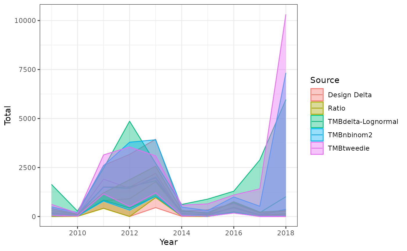
The results from multiple runs can also be combined, with bind_rows.
Run1<-loadOutputs(baseDir = getwd(),
                  runName = "Run1",
                  designScenarios = c("noPool","Pool1"),
                  modelScenarios = c("s1","s2"))
Run2<-loadOutputs(baseDir = getwd(),
                  runName = "Run2",
                  designScenarios = c("noPool","Pool1"),
                  modelScenarios = c("g1","g2"))
allRuns<-bind_rows(Run1,Run2)
This code will produce a data frame with all the results from all scenarios and species in both runs together, distinguished by the column called “Run”.
Within the list returned by loadOutputs,the results
under designOutputs and modelOutputs include:
ModFits, a list for all species, containing lists of all model fits.
modpredVals, a list for all species, containing a list of tibbles of the bycatch.
allmods, a long format tibble with all the model annual predictions together, which is included in allYearEstimates
Allindex, the same for abundance indices if calculated.
And for design-based results:
designyeardf, the annual estimate of bycatch, the same as the .csv file
poolingSum, the pooling summary data, the same as the .csv file
yearSumGraph, annual summaries in the same formula as the model outputs in allmods, which are combined in allYearEstimates
Validation and conclusions
Although this code automates much of the process of bycatch estimation, including model selection, it is important to keep in mind that the results are only correct if the assumptions of the method are met. All methods of expanding a sample (e.g. observer data) to the total fishery (e.g. logbooks) are dependent on the assumption that the sample is representative of the whole fishery. This assumption may be violated in many cases because, for example:
Only certain kinds of vessels take observers (e.g. only larger vessels have room for observers, some ports or sectors are more cooperative).
Fishers behave differently when observers are present, for example avoiding bycatch if observer data is used for enforcement.
The observer program allocates observers non-randomly, without adequately documenting the allocation criteria, or how the allocation has changed over time.
Observer data includes information from extra trips, above the usual observer monitoring, that were specifically targeted for some research purpose, e.g. a bycatch mortality study, or extra trips in a strata where bycatch was known to be a problem.
Observer data is combined from multiple sources, and it is not clear which components of the fishery are covered by each (e.g. observers placed by different programs for different gear or target species, but some vessels participate in both).
Total effort data is not representative of the fishery, for example because not all fishers report their effort, or the effort is inferred from landings records, or the units of effort are not interpreted the same way in logbooks vs. observer data.
For all of these reasons, it’s important to validate bycatch estimates if possible. One possible validation technique is to use the bycatch estimate method to estimate the total catch of landed species, and compare them to total landings. If the total landings of several target species estimated by the bycatchEstimtor tool are consistent with the recorded landings weighed at fish landing sites, then this indicates that the observer data are representative of the fishery. If the estimates are not consistent with the known landings, then one of the problems listed above may exist. In some cases including additional stratification or predictor variables may resolve the problem (e.g. vessel size, or an indicator variable for different observer programs with different sampling strategies).
For model-based estimation, it is not recommended that the final model be used without looking closely at the outputs. The selected model must have good fits and should be reasonably consistent with data according to the DHARMa residuals. The results should appear reasonable and be around the same scale as the ratio estimator results. The model should not be overly complex. Also, look at the model selection table to see if other models are also supported by the data. If model-based estimates are very different from design-based estimates, it is important to understand why they differ. In some cases, model results using additional variables (e.g. variables giving more details on fishing gear or fish habitat), the model-based estimates may be better. For more guidance on bycatch estimation, see the simulation papers published at ICCAT (Babcock et al. (2022), Babcock et al. (2023)).
Appendix
Descriptions of columns for outputs from each function.
bycatchSetup function
DataSummary/StrataSummary tables:
- Year
- Eff: effort in logbook data
- Units: sample units in logbook data
- OCat: observed catch (observer data)
- OEff: observed effort (observer data)
- Ounit: observed sample units (observer data)
- CPUE: mean catch per unit effort
- CPse: standard error of CPUE
- Out: count of outliers defined as data points more than 8 SD from the mean
- Pos: number of sample units with positive observations (presence)
- OCatS: standard deviation of observed catch
- OEffS: standard deviation of observer effort
- Cov: covariance matrix
- PFrac: fraction of positive observations (positive observations divided by observed sample units)
- EFrac: fraction of effort observed (observed effort divided by logbook effort)
- UFrac: fraction of sample units observed (observed sample units divided by logbook sample units)
- Cat: estimated catch using unstratified ratio estimator (observed catch divided by observed effort raised by logbook effort)
- Cse: standard error of estimated catch
bycatchDesign function
Pooling.csv file:
- Year
- totalUnits: sum of sample units in logbook data
- totalEffort: sum of effort in logbook data
- units: sum of sample units in observer data
- effort: sum of effort in observer data
- pooled.n: number of sample units that don’t need pooling (observer sample units > minStrataUnit)
- poolnum: number of sample units where pooling occurred?
- pooledTotalUnits: pooled total sample units (logbook data)
- pooledTotalEffort: pooled total effort (logbook data)
DesignYear/DesignStrata tables:
- Year
- ratioMean: mean bycatch calculated by the ratio estimator
- ratioSE: standard deviation of the ratio estimator
- deltaMean: mean bycatch calculated by the delta estimator
- deltaSE: standard deviation of the delta estimator
bycatchFit function
AnnualSummary/StratumSummary tables:
- Year
- Total: estimated total bycatch
- Totalvar: variance of estimated total bycatch
- Total.mean: mean across simulations (only when VarCalc = Simulate)
- TotalLCI: lower confidence interval bound
- TotalUCI: upper confidence interval bound
- Total.se: standard error of estimated total bycatch
- Total.cv: coefficient of variation
ModelSelection tables:
- cond..Int: intercept of conditional model
- disp..Int: intercept of dispersion model
- AICc, AIC, BIC: model information criteria (lower is better)
- df: degrees of freedom
- logLik: log-likelihood of the model
- selectCriteria: criteria actually used to rank the models
- delta: difference in the selection criteria from the best model
- weight: Akaike weights (relative support for each model)
Index tables:
- Index: mean cpue
- SE: standard error of mean cpue
- lowerCI: lower bound of confidence interval
- upperCI: upper bound of confidence interval
crossvalSummary table:
- model: model type
- formula: formula of BIC best model
- RMSE: root mean square error
- ME: mean error
modelSummary table:
- KS.D: value of Kolmogorov-Smirnov test of uniformity of residuals
- KS.p: p-value of Kolmogorov-Smirnov test of uniformity of residuals
- Dispersion.ratio: value of dispersion test (residuals variance), which compares the ratio between observed and simulated residuals
- Dispersion.p: p-value of dispersion test
- ZeroInf.ratio: value of zero inflation test which compared ratio of observed and expected zeros
- ZeroInf.p: p-value of zero inflation test
- Outlier: outlier test, number of residuals that are outside expected 95% confidence interval
- Outlier.p: p-value for outlier test
me and rmse tables:
- values of mean error (ME) and mean square error (RMSE) for each fold of cross validation